Sending a swarm of LLM agents to predict the 2026 US midterm elections

You can explore the live 2026 House and Senate forecast and the interactive voter swarm at electionprediction.martinsiron.com.

Ten years ago, during the 2016 primaries, I wrote a post on this blog trying to predict the remaining Democratic primary contests using a spreadsheet of state demographics, primary rules, and a few linear regressions. It was a very simple setup (I even had to throw out Vermont with a Dixon Q-test because Bernie Sanders was such an outlier in his home state), and by some luck it called Indiana within two points a few days later.

With the 2026 midterms coming up on November 3, I wanted to revisit election modeling with a more serious setup. In particular, I wanted to compare two different ways of modeling an election on top of the same underlying data lake: a classical top-down statistical Monte Carlo model and a bottom-up agent-based microsimulation. I also wanted to test a question that has been getting a lot of attention in computational social science lately: if you populate an agent-based model with large language model (LLM) voter personas reading campaign news and arguing with their neighbors, does it actually help forecast an election, or does it mostly reflect the biases baked into the language models?

Everything is live at electionprediction.martinsiron.com. Below is a walkthrough of how the data lake is structured, how the two models work, what data they share (and do not share), and some strange racial and educational biases that showed up when testing the LLM voter agents.

Top-down vs. bottom-up election forecasting

Most quantitative election forecasts in political science and data journalism follow a top-down hierarchy. In the classic "fundamentals plus polls" literature, such as Alan Abramowitz's Time for Change model or Bafumi, Erikson, and Wlezien's work on generic-ballot balancing in midterm elections, you start with a national barometer of the political environment (like the national generic congressional ballot), anchor each state or congressional district on its prior presidential vote share and incumbency, blend in race-specific polling where available, and simulate correlated national, state, and race-level errors. Modern hierarchical Bayesian and Monte Carlo forecasts, such as Gelman, Heidemanns, and Morris (2020) for The Economist or FiveThirtyEight's congressional models, add richer covariance structures across states, but the core logic remains top-down: the unit of analysis is the aggregate jurisdiction (the state or congressional district), and national or regional swings are pushed down onto those jurisdictions.

A bottom-up microsimulation (or agent-based model) starts from the opposite end. Instead of treating a county or district as a single number, you construct a synthetic population of eligible voters stratified by race and educational attainment, assign each subgroup its empirical turnout propensity and party vote probability from individual-level survey microdata, let those synthetic voters interact inside a local social network, and aggregate their simulated ballots back up into counties, congressional districts, and states.

Neither approach is guaranteed to beat the other. Top-down models have the advantage that a district's past election return already captures local political culture and unmeasured factors that demographic tables miss. Bottom-up models make it possible to decompose a shift by turnout versus persuasion across specific demographic subgroups, though they have to deal with survey sampling noise in small rural counties. Building both on the same data lake made it possible to test them side by side on historical elections from 2012 to 2024 before making a 2026 projection.

Engineering the data lake: tracking voters across redrawn boundaries

When you build a House forecast from raw data rather than downloading a pre-compiled spreadsheet, the first real engineering hurdle is redistricting. Between 2022 and 2026, court rulings and legislative redraws altered congressional boundaries in North Carolina, Alabama, Louisiana, Georgia, Texas, Ohio, and New York. Professional forecasters and election data teams (such as The Downballot / Daily Kos Elections, FiveThirtyEight, Split Ticket, and The New York Times) handle this by disaggregating prior election returns down to the voting precinct or Census block and re-summing them inside the new district boundaries.

To do that reproducibly across four different congressional map vintages (the 116th, 118th, 119th, and 120th Congresses, so that our 2018 and 2022 midterm backtests use the exact boundaries those elections were fought on), the geospatial pipeline is built around one rule: a district's identity in the data lake is its geographic polygon in a given Congress, never its district number.

1. Equal-area precinct projection: We ingest precinct-level shapefiles and returns from the Voting and Election Science Team (VEST) for 2016 and 2020, and the New York Times precinct compilation for 2024. Because state precinct files arrive in a mix of coordinate systems, every layer is first projected into a common equal-area projection (Conus Albers Equal Area). For each precinct polygon, we compute an interior representative point (which is guaranteed to lie inside concave or multi-part precincts, unlike a geometric centroid) after projecting, and spatially join those points against the Census TIGER congressional district polygons for the target Congress.
2. Statewide reconciliation and county fallback: After summing precinct votes into districts, each state is checked against certified statewide returns from the MIT Election Data and Science Lab (MEDSL). Where a raw precinct file has a hole (for example, the 2024 precinct compilation is missing Oklahoma and Tulsa counties, which account for 35% of Oklahoma's vote and its two most Democratic urban centers), the pipeline flags the discrepancy and repairs the missing district totals by allocating certified county returns through a county-to-district crosswalk.
3. Vote-weighted vs. area-weighted crosswalks: We also build crosswalks between counties and districts and between successive congressional maps to project county-level demographic swings onto House seats and to track territorial incumbency (if a redrawn 2026 district takes more than half of its voters from an incumbent's 2024 district, it inherits that incumbency advantage even if the district number changed). Initially, I weighted polygon intersections by land area. That turned out to be a terrible idea whenever a boundary cut across a dense city and its rural suburbs: in metro Atlanta, splitting the 2022 GA-06 and GA-07 districts onto the redrawn GA-06 and GA-07 boundaries by land area produced a 51-point error (81.9% vs. 31.0% actual). Replacing land area with the two-party votes cast at the precinct points inside each intersection fragment cut that error from 51 points to 1.1 points.

What data do the two models share, and where do they differ?

A fair question is whether the two models are just repackaging the exact same inputs. They share the same foundational geography and polling tables in the lake, but they use completely different demographic, survey, and variance inputs:

Data Layer / Feature	Top-Down Monte Carlo	Bottom-Up Voter Swarm
Precinct-reaggregated 2024 presidential baseline	Yes (starting baseline for each House seat)	Yes (combined with crosswalked county swarm shift)
Vote-weighted territorial crosswalks	Yes (maps county swing and territorial incumbency to seats)	Yes (aggregates simulated counties into 2026 districts)
National generic ballot	Yes (de-biased exponential-decay average sets national shift)	Yes (anchors the national environment for 2026 midterm runs)
Live 2026 district & state polls	Yes (blended on logit scale after national shift)	Yes (blended into district and state projections)
Incumbency & 6-year Senate seat history	Yes (territorial House bonus; historical 6-year Senate seat overperformance)	Yes (adopted after cutting out-of-sample Senate call errors in half)
Expert race ratings (Cook, Inside Elections, Sabato, DDHQ)	Yes (residual of consensus rating on presidential lean)	Yes (residual surprise term used in Congress roll-ups; not used in county or state presidential swarm)
County Census / BEA macro covariates	7 covariates fitted on between-election swing (Δ logit)	11 covariates (adding poverty, white × college interaction, and multiracial share) fitted as a multilevel prior with James-Stein state random intercepts
Census Citizen Voting-Age Population (CVAP) race × education cells	Not used (except state non-college white share as a single composition axis)	Core skeleton: partitions all 3,112 counties into 10 race × college strata (~1.56M synthetic voter nodes)
Cooperative Election Study (CES) individual microdata (N = 718,955)	Not used	Core behavioral input: estimates validated voter-file turnout and subgroup log-odds vote offsets across 126,771 validated voters
Social network & LLM voter dialogues	Not used	Used in Swarm: small-world homophily graph with Friedkin-Johnsen logit opinion dynamics and LLM conversation calibration

How the Top-Down Monte Carlo model works: measuring the shift and its uncertainty

In the Top-Down model (/forecast.html), the mathematical question we are asking for each of the 435 House districts is: Starting from the 2024 two-party presidential vote cast inside this district's 2026 boundaries, how far should we shift its log-odds (logit(p) = ln(p / (1 − p))) for the 2026 midterm environment, and how much correlated versus idiosyncratic uncertainty surrounds that point estimate?

Working on the log-odds scale is standard in political methodology because a uniform additive shift in log-odds naturally compresses near 0% and 100% rather than pushing safe seats past 100% or below 0%. For district d in state s, the model builds the central log-odds prediction μ_d and simulates its uncertainty in five steps, with all blending weights and shrinkage parameters chosen by out-of-sample forward-chaining (training strictly on cycles before t and scoring on cycle t via log loss):

1. Between-county demographic swing: Rather than regressing election levels on demographics (where the lagged election result swallows almost all the variance), we fit weighted least squares on the change in county log-odds between elections, Δℓ_c = logit(D_c,t) − logit(D_c,t−1), across standardized county covariates (bachelor's degree share, racial composition, population density, unemployment, and income). Because demographic realignment trends occasionally slow down or flip sign across eras, the slope vector is partially pooled between the most recent cycle and the full historical panel, scaled by how strongly demographic shifts predicted county movement in the preceding cycle, centered to zero national mean, and projected onto congressional districts via the vote-weighted crosswalk.
2. District fundamentals (incumbency, educational composition, and rating surprise): To the district's 2024 presidential baseline and demographic swing, we add a territorial incumbency bonus (plus a 6-year seat overperformance term in the Senate that captures incumbents like Susan Collins or Joe Manchin who consistently outrun their state's presidential lean), a state educational-composition offset learned from prior midterms, and an expert rating residual. Adding raw race ratings from Cook, Inside Elections, Sabato, and DDHQ directly to a district's lean would double-count the presidential baseline and artificially narrow the seat distribution, so we regress the expert consensus on the presidential lean within the current cycle and add only the residual (the local candidate quality or retirement signal that the baseline misses).
3. De-biasing the generic ballot and solving for the national shift: To anchor the overall midterm wave, we compute an exponentially time-decayed average of national generic-ballot polls. As of October 21, 2026, the raw generic-ballot average puts Democrats at 54.0% of the two-party vote (D+8.0). However, when we replay that exact same estimator across all 14 cycles since 1998, it overstated Democrats in 11 of 14 cycles, and by an average of 1.7 percentage points of two-party share (3.5 points of margin) across the 7 midterms. Subtracting that historical midterm bias brings the 2026 national target to 52.3% Democratic (D+4.5). We then use bisection to solve for the single uniform shift δ_nat such that the turnout-weighted national vote across all 435 districts lands exactly on the target:

   ∑_d=1..435 w_d expit(ℓ_d^pre + δ_nat) / ∑_d=1..435 w_d = p_target (Solving by bisection rather than taking a simple difference of logits matters because, by Jensen's inequality, a vote-weighted average of nonlinear logistic curves compresses the shift enough to miss by about two House seats.)

4. Blending live district and state polls after the national shift: For races with live 2026 polling averages, we blend the race's polling log-odds with the shifted fundamentals:

   μ_d = (1 − w_d)(ℓ_d^pre + δ_nat) + w_d logit(p̄_d^poll) Order of operations is critical here: if you blend district polls before solving for δ_nat, you apply the national wave a second time on top of polls that already reflect the 2026 environment, while forcing the solver to push the unpolled districts in the opposite direction.

5. Simulating 40,000 elections with four variance components: In each of the 40,000 Monte Carlo runs, district d's realized two-party Democratic share is drawn by adding four normal shocks on the log-odds scale before mapping back to probability via expit:

   p_r,d = expit(μ_d + ε_r^nat + ε_r,s(d)^state + z_s(d) ε_r^axis + ε_r,d^seat)

   • A national shock ε_r^nat shared by all 435 seats, calibrated from the historical residual standard deviation of our generic-ballot estimator across past midterms (accounting for roughly three-fifths of total seat-count variance).
   • A state shock ε_r,s^state shared by all districts in state s, calibrated from historical state-level midterm residuals.
   • A correlated demographic-composition shock z_s(d) ε_r^axis scaling with state s's standardized white non-college share z_s. In 2016, a single regression of state polling error on white non-college share explained 59% of the cross-state error variance, yet the sign of that error flipped by 2024. Drawing one axis shock per simulated election means we do not pretend to know which way that demographic group will break in 2026, but if it breaks, exposed states like Michigan, Wisconsin, Pennsylvania, and Ohio move together rather than independently.
   • A heteroskedastic district shock ε_r,d^seat whose standard deviation grows linearly with how far a seat is from 50-50. In our 2018 and 2022 House backtests, safe seats had more than twice the residual variance of toss-up seats (because safe races often feature token opposition or blowouts, whereas toss-ups attract heavy spending on both sides).

How the Bottom-Up Voter Swarm model works

The Bottom-Up Voter Swarm (/swarm_atlas.html) asks whether we can recover state and congressional election outcomes by building the electorate from the ground up out of demographic subgroups:

1. County demographic skeleton: For each of 3,112 U.S. counties, we cross Citizen Voting-Age Population (CVAP) race counts (white, black, hispanic, asian, other) with the county's bachelor's degree share into 10 race × college cells, expanding each cell into 50 synthetic voter personas (up to 500 per county, or ~1.56 million nationally), each weighted by the number of voting-eligible citizens it represents.
2. Survey-validated subgroup baselines: Using the cumulative Cooperative Election Study (CES, 718,955 total respondents; 126,771 validated general-election voters in 2016, 2020, and 2024), we measure each cell's validated voter-file turnout rate (using Catalist voter-file validation rather than self-reported turnout, which is heavily over-reported in surveys) and its subgroup log-odds offset Δ_g^CES relative to the national electorate.
3. Recentering on an out-of-sample multilevel county prior: Applying national subgroup vote shares directly to every county would treat rural Wyoming white non-college voters and urban Massachusetts white non-college voters as identical, while adding subgroup offsets on top of a county regression would double-count demography. Instead, we fit an out-of-sample weighted least-squares multilevel model of county log-odds on lagged county vote, 11 county covariates, and James-Stein empirical Bayes shrunk state random intercepts, and then use bisection inside each county c to solve for the shift δ_c such that the turnout-weighted sum of the 10 subgroups matches the county's prior expectation p̂_c^prior:

   ∑_g=1..10 N_c,g t_c,g expit(Δ_g^CES + δ_c) / ∑_g=1..10 N_c,g t_c,g = p̂_c^prior Individual personas in cell g then draw their baseline vote probability and turnout propensity from Beta distributions centered on those rescaled subgroup means.

4. Friedkin-Johnsen peer network dynamics: Within each county, personas are connected in a small-world homophily graph (k = 12 neighbors per node, with higher within-group connection probability and 10% random long-range rewiring). Over successive rounds of social interaction, persona i updates its log-odds opinion q_i = logit(p_i) as a weighted average of its own initial anchor q_i⁽⁰⁾ and its neighbors' opinions, governed by its individual social susceptibility β_i (Friedkin and Johnsen 1990):

   q_i^(k+1) = (1 − β_i) q_i⁽⁰⁾ + β_i ∑_j W_ij q_j^(k)

Out-of-sample backtests: does bottom-up beat top-down?

Every model component was evaluated using strict forward-chaining, anchored on the archived election-eve national polling average rather than the realized national vote:

Benchmark (Out-of-Sample)	Units Scored	Bottom-Up Swarm Calls	Top-Down MC Calls	Swarm MAE	Top-Down MAE
2012-2024 President (4 cycles)	204 state-cycles	198 / 204 (97.1%)	196 / 204 (96.1%)	1.76 pp state / 3.02 pp county	2.93 pp county (1.31 pp in 2024)
2018 House Midterms	393 districts	377 / 393 (95.9%)	383 / 393 (97.5%)	2.58 pp	3.70 pp
2022 House Midterms	398 districts	382 / 398 (96.0%)	385 / 398 (96.7%)	2.09 pp	2.53 pp
2018-2022 / 2024 Senate	92 / 130 races	125 / 130 (96.2%)	85 / 92 (92.4%)	Brier 0.0365	2.31 pp (Brier 0.0497)

In the presidential backtest, the Bottom-Up Swarm edges out the Top-Down model across the four cycles (198/204 vs. 196/204, including a 51/51 sweep in 2024), while in the 2018 and 2022 House midterms the Top-Down model calls 3 to 6 more winners even though the Swarm achieves slightly lower district vote-share MAE (2.09 pp vs. 2.53 pp in 2022). Notably, when we first tried rolling the Bottom-Up county swarm directly up to House districts without anchoring each district on its precinct-scored presidential baseline, it missed 53 House seats in 2018 and 64 in 2022 (6.18 pp and 5.70 pp MAE), because in multi-district urban counties like Los Angeles, Cook, or Maricopa, a county-wide demographic average cannot tell which neighborhoods were packed into a safe seat versus a swing seat. Combining the precinct-scored district baseline with the crosswalked county swarm swing cut those House call errors from 117 down to 32 across the two midterms.

Testing LLM voter agents: silicon sampling, racial biases, and peer backfire

Over the past three years, a growing body of political science and machine learning research has explored whether large language models conditioned on demographic personas can stand in for human survey respondents. Argyle et al. (2023) coined the term "silicon sampling", showing that GPT-3 conditioned on American National Election Studies (ANES) backstories reproduced many aggregate partisan correlations. Subsequent studies, however, raised serious warnings: Santurkar et al. (2023) and Bisbee et al. (2024) found that LLM personas suffer from variance collapse (regressing toward caricatured group stereotypes with far less within-group diversity than real voters) and shift unpredictably across prompts and models, while Chuang et al. (2024) studied how networks of LLM agents polarize or converge during multi-turn political discussions.

To test these ideas directly against our data lake, we pulled 471,457 dated New York Times articles from 2010 to 2026 via the NYT Archive API, built strictly date-bounded 40-item campaign news digests (restricted to articles published before T − 180, T − 112, T − 56, and T − 21 days before each election), and drew 17,850 synthetic voter evaluations across five election cycles (2012, 2016, 2020, 2024, 2026) using two models (google/gemini-2.5-flash-lite and openai/gpt-oss-120b), plus 175 four-turn neighbor-to-neighbor political conversations (700 dialogue turns).

When we compared the LLM voter personas directly against the 126,771 validated voters in the Cooperative Election Study (CES), three striking racial and educational biases emerged:

Demographic Subgroup (race:education)	CES Validated Voters (N = 126,771) Log-Odds Lean	LLM (Gemini 2.5) 2024 Log-Odds Lean	LLM (GPT-OSS-120B) 2024 Log-Odds Lean	LLM (Gemini 2.5) Mean P(Dem) / Strict D%	LLM (Gemini 2.5) Undecided %	CES Validated vs. LLM Turnout
Black · College	+2.039 (~89.6% D)	+1.423	+1.411	0.792 / 97.9%	12.7%	59.2% vs. 87.7%
Black · Non-college	+2.010 (~89.3% D)	+0.912	+1.181	0.695 / 100.0%	32.8%	42.7% vs. 75.5%
Asian · College	+0.870 (~72.7% D)	+1.098	+1.137	0.733 / 100.0%	22.7%	49.9% vs. 85.1%
Asian · Non-college	+0.438 (~63.4% D)	+0.410	+0.379	0.580 / 88.4%	44.4%	33.6% vs. 65.6%
Hispanic · College	+0.580 (~66.7% D)	+0.767	+1.024	0.664 / 86.8%	35.6%	54.1% vs. 81.9%
Hispanic · Non-college	+0.572 (~66.5% D)	+0.005	+0.174	0.480 / 59.4%	61.4%	38.5% vs. 66.0%
White · College	+0.185 (~57.0% D)	+0.062	+0.160	0.494 / 53.0%	19.9%	73.9% vs. 83.6%
White · Non-college	-0.572 (~38.8% D)	-0.617	-0.714	0.331 / 19.4%	38.1%	57.6% vs. 70.0%

1. The LLMs project the white "diploma divide" onto Black and Hispanic voters: In actual validated voter records (CES), educational polarization is overwhelmingly a white phenomenon: college-educated white voters are 0.76 logits (~18 percentage points) more Democratic than non-college white voters (+0.185 vs. -0.572). Among Black and Hispanic voters in the CES, college and non-college voters cast Democratic ballots at almost identical rates (+2.039 vs. +2.010 for Black voters; +0.580 vs. +0.572 for Hispanic voters). Both LLMs, however, hallucinate a massive educational chasm inside non-white racial groups. In 2024, gemini-2.5-flash-lite puts college-educated Hispanic voters at +0.767 logits (mean P(Dem) = 0.664) while dropping non-college Hispanic voters to +0.005 (P(Dem) = 0.480), and creates a 0.51-logit gap between college and non-college Black voters (+1.423 vs. +0.912, widening to +1.426 vs. +0.663 in 2026). The language models appear to have learned a blanket rule from post-2016 political commentary that "non-college working-class voters lean Republican" and over-applied it mechanically across every race.
2. Discrete stereotyping vs. continuous probability hedging on Black voters: When forced to pick a discrete ballot (D or R), gemini-2.5-flash-lite exhibits classic variance collapse: among decided Black personas, it assigns 100.0% Democratic to college-educated Black personas in 2012, 2016, 2020, and 2026 (97.9% in 2024) and 100.0% Democratic to non-college Black personas in 2024, erasing the ~10% of Black voters who vote Republican in validated data. Yet when asked in the very same response for a continuous vote probability, the model hedges non-college Black personas down to 0.695 in 2024 and 0.619 in 2026, pulling their continuous expectation nearly 20 points below the empirical CES rate.
3. Treating non-college Hispanic voters as chronically "undecided" while inflating turnout: Even 21 days before the election, the LLM marks 52% to 61% of non-college Hispanic personas as undecided across every cycle from 2012 to 2026 (compared to 0% to 13% for Black college personas and 10% to 20% for white college personas). At the same time, just like human survey respondents exhibiting social-desirability bias, the LLM personas over-report turnout by 27 to 33 percentage points among lower-propensity non-white non-college groups (66% to 76% LLM turnout vs. 34% to 43% validated voter-file turnout in CES).

We also ran a contamination check asking the LLM to estimate the national two-party vote across four experimental arms: blind (given only the election date, with zero news), digest (given the dated NYT digest), polls (digest + polling average), and suppressed (explicitly instructed to set aside hindsight). In blind mode, with no news at all, the model recalled 0.5203 for 2012 (0.5196 certified) and 0.4950 for 2024 (0.4925 certified), while in 2016 it guessed 0.4820 (0.5108 certified), confusing Donald Trump's Electoral College victory with the national popular vote.

Because of both findings (hindsight recall on past cycles and the racial/educational distortions in raw LLM subgroup leans), we do not let raw LLM vote shares set the level of any county or district in the production forecast. Our county recentering step guarantees by construction that county levels stay anchored to the out-of-sample statistical prior, and in our ablation tests, replacing the empirical CES subgroup offsets with LLM subgroup offsets did not beat the CES baseline.

Where the LLM agents do provide a clean measurement that no historical table in our data lake can supply is in calibrating the social-network parameters. In the Friedkin-Johnsen network equation, two parameters had previously been unmeasured guesses: individual social susceptibility β_i (originally assumed to average 0.30) and within-cell homophily (originally assumed to be 6.0). Because the two-person Friedkin-Johnsen update in logit space is q_after = (1 − β_i) q_before + β_i q_other, we can measure β̂_i directly by probing two LLM voter personas privately before and after a 4-turn political conversation on the 2026 cycle (where no election outcome exists in any model's weights):

β̂_i = [logit(p_after,i) − logit(p_before,i)] / [logit(p_before,other) − logit(p_before,i)]

Across 175 four-turn conversations (100 pairs on gemini-2.5-flash-lite and 75 pairs on gpt-oss-120b, stratified across four pairing buckets), here is what the dialogues produced:

Conversation Bucket (2026 Cycle, 700 Turns)	Pairs (N)	Positive Susceptibility β̂+	Raw Clipped β̂	Mean |ΔP(Dem)|	Backfire Rate (β̂ < −0.01)
Bucket A · Same demographic cell, same party lean	46	0.089	-0.061	2.9%	43.6%
Bucket B · Different cell, same party lean	45	0.151	-0.043	3.2%	50.0%
Bucket C · Same demographic cell, opposite party lean	42	0.039	-0.024	3.0%	45.2%
Bucket D · Different cell, opposite party lean	42	0.039	-0.025	3.0%	47.6%
Pooled across all 175 pairs (350 agent probes)	175	0.079	-0.037	3.0%	46.4%

Two findings stood out from the conversation transcripts:

• Persuasion is small and backfire is common: Positive susceptibility averaged just β̂₊ = 0.079 across the two models (0.049 on Gemini 2.5 Flash-Lite, 0.118 on GPT-OSS-120B, with a pooled median of 0.000), roughly a quarter of the 0.30 prior we had initially assumed. In nearly half of cross-party arguments (45.2% in Bucket C and 47.6% in Bucket D), arguing with an opposite-party neighbor caused agents to dig in slightly harder on their initial view (β̂_i < −0.01).
• Demographic homophily did not increase persuadability: Comparing same-cell conversations (Buckets A + C, β̂₊ = 0.063) against cross-cell conversations (Buckets B + D, β̂₊ = 0.094) gave a homophily ratio of 0.675, well below the assumed 6.0. Reading the private post-conversation thought logs shows why: once a persona is anchored on concrete household concerns (grocery prices, insurance premiums, local hospital closures, or border policy), sharing a demographic label with an interlocutor does very little to soften partisan disagreement.

Where the 2026 midterm race stands

Putting all of this together, both models currently point to a clear Democratic advantage in the U.S. House and a narrow, toss-up-leaning-Democratic battle for the U.S. Senate.

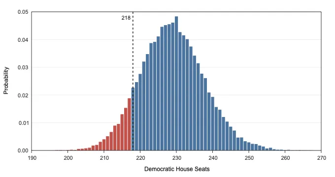
In the U.S. House (218 seats needed for a majority), the raw generic-ballot polling average sits at 54.0% Democratic (D+8.0), which our historical midterm bias correction adjusts down to 52.3% Democratic (D+4.5). Even after that 3.5-point margin haircut, the national environment is favorable enough for Democrats that the two models land within half a seat of each other:

• Top-Down Monte Carlo: 229.6 D - 205.4 R (91.9% probability of a Democratic majority; 80% interval 218 to 241 D, 95% interval 213 to 248 D).
• Bottom-Up Voter Swarm: 230.0 D - 205.0 R (92.1% probability of a Democratic majority; 80% interval 219 to 242 D, 95% interval 213 to 249 D).

Control of the House runs through roughly 30 competitive districts where the 80% simulation interval spans both sides of 50%, including MI-04 (Kalamazoo), ME-02 (Northern Maine), NY-17 (Hudson Valley), CO-08 (North Denver), AZ-06 (Tucson East), MI-07 (Lansing), IA-01 (Davenport), and PA-07 (Lehigh Valley).

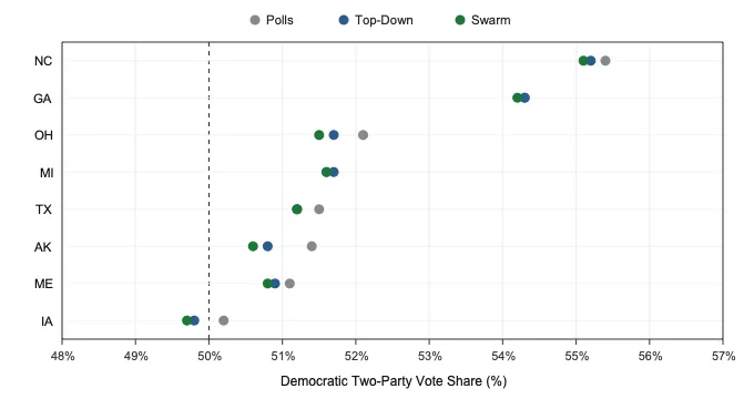
In the U.S. Senate (51 seats needed for a majority), 35 seats are on the ballot: the 33 regular Class 2 seats plus the special elections in Florida and Ohio to fill the seats vacated by Marco Rubio and JD Vance. Democrats hold 34 of the 65 seats not up this cycle (including the two independents, Bernie Sanders and Angus King, who caucus with them), so they need to win 17 of the 35 races on the ballot to reach 51 seats:

• Top-Down Monte Carlo: 51.2 D - 48.8 R (17.16 of the 35 seats on the ballot; 60.9% Democratic majority probability; 80% interval 48 to 54 D).
• Bottom-Up Voter Swarm: 51.0 D - 49.0 R (16.97 of the 35 seats on the ballot; 58.2% Democratic majority probability; 80% interval 48 to 54 D).

As the figure above shows, the Senate majority hinges on eight competitive states where state-level polls and structural fundamentals sometimes pull in different directions: North Carolina, Georgia, Ohio (Special), Michigan, Texas, Alaska, Maine, and Iowa. Notice how both models pull strong Democratic polling averages in historically Republican-leaning states like Texas, Alaska, and Ohio back toward 50% once 2024 presidential lean and seat history are factored in, while keeping Maine tight because of Susan Collins's historical six-year seat overperformance.

Current 2026 Forecast (Live Widget)

The table below automatically pulls the latest published run from electionprediction.martinsiron.com whenever the models re-run between now and Election Day:

Last updated: October 21, 2026 (open live dashboard)

Chamber & Model	Projected Seats (Mean)	80% Interval (p10-p90)	P(Dem Majority)	Interactive View
U.S. House · Top-Down Monte Carlo	229.6 D - 205.4 R	218 - 241 D	91.9%	Simulator
U.S. House · Bottom-Up Voter Swarm	230.0 D - 205.0 R	219 - 242 D	92.1%	Swarm Atlas
U.S. Senate · Top-Down Monte Carlo	51.2 D - 48.8 R	48 - 54 D	60.9%	Simulator
U.S. Senate · Bottom-Up Voter Swarm	51.0 D - 49.0 R	48 - 54 D	58.2%	Swarm Atlas

If you want the final locked-in numbers the day before the election, you can sign up here for the Election-Eve Dispatch: I will send out a single email on November 2, 2026 with the final House and Senate calls from both models (one email only, zero spam). And if you enjoy exploring the voter swarm, the methodology sandbox, or this write-up and want to help cover the compute and hosting costs, you can buy me a coffee here.

We will see on November 3 how both models hold up against the real electorate!